

It has been too long since I last studied, so let me review. These are notes taken with reference to the study video
Huawei Data Communication
Network Models
OSI Model
-
Application Layer (Layer 7)
- Provides interfaces and services to applications
-
Presentation Layer
- Performs data format conversion, encryption and decryption, and image/text encoding
-
Session Layer
- Establishes, maintains, and terminates communication sessions
-
Transport Layer
- End-to-end transmission; responsible for ports and reliable/unreliable transmission
-
Network Layer
- Routing and addressing; determines the data path
-
Data Link Layer
- Transmission between adjacent devices, error checking, physical addressing
-
Physical Layer (Layer 1)
- Physical hardware, signal transmission; only transmits the bit stream of 0/1
TCP/IP Model
-
Application Layer (Layer 4)
-
Combines the OSI application, presentation, and session layers. Faces users and programs
-
Protocols: HTTP (80), HTTPS (443), FTP (21), SSH (22), Telnet (23), SMTP (25), POM3 (110), IMAP (143), DNS (53), apps and browsers, etc.
-
-
Transport Layer
-
End-to-end transmission; distinguishes programs by port
-
Protocols: TCP (0
65535) reliable, UDP (065535) efficient -
0~1023 are well-known fixed ports, 1024+ are dynamic custom ports
-
-
Internet Layer (Internetwork Layer)
-
Routing and addressing; finds the destination host by IP address
-
Protocols: IP, ICMP
-
-
Network Interface Layer (Network Layer)
-
Combines the OSI data link layer and physical layer; responsible for hardware transmission, MAC addressing, and cable/signal forwarding
-
Devices: network interface cards, switches, cables
-
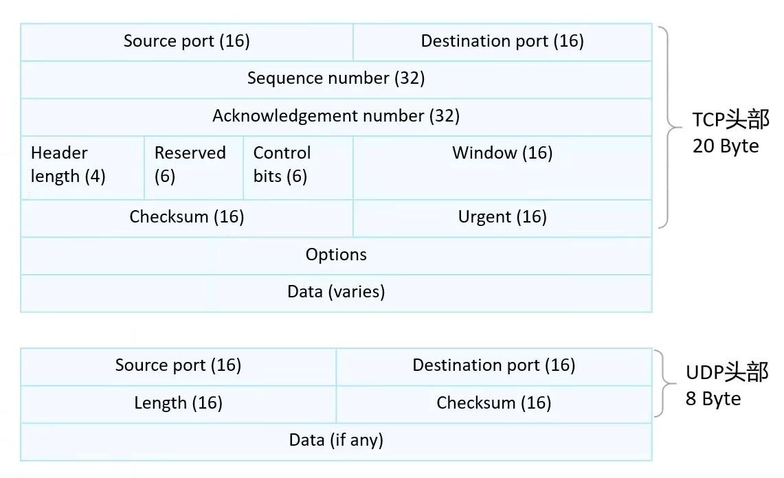
TCP/UDP Packet Format
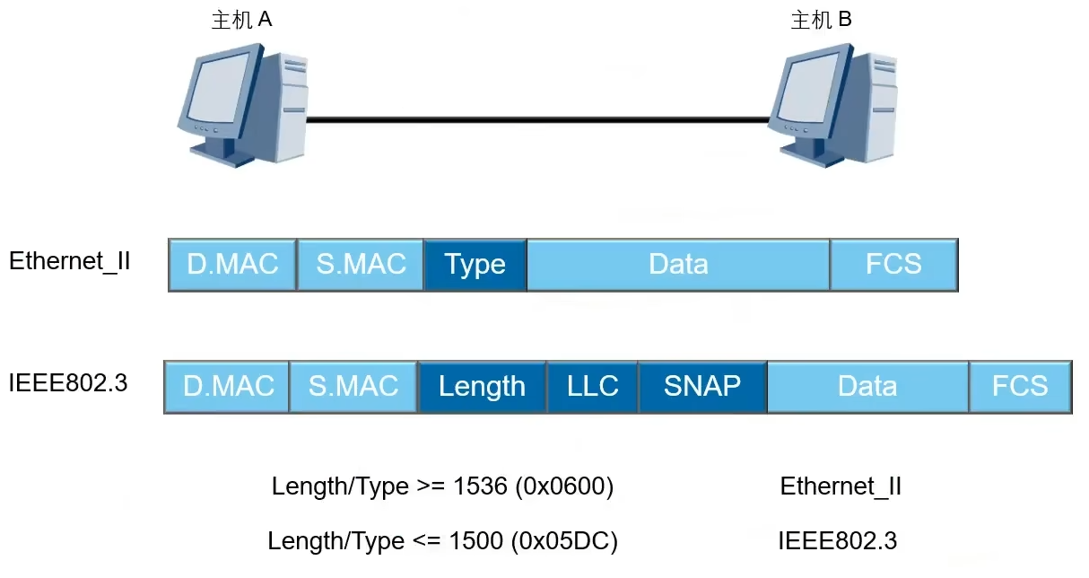
Ethernet Frame Format
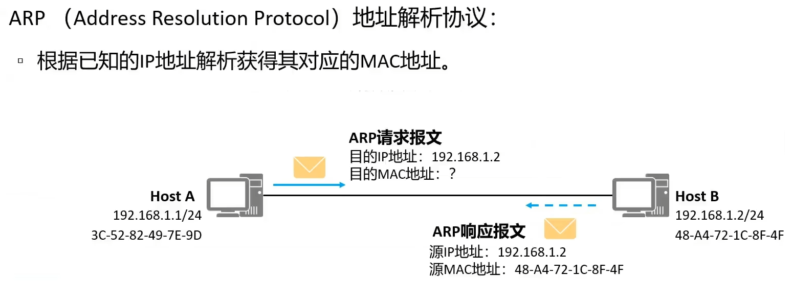
ARP Address Resolution Protocol
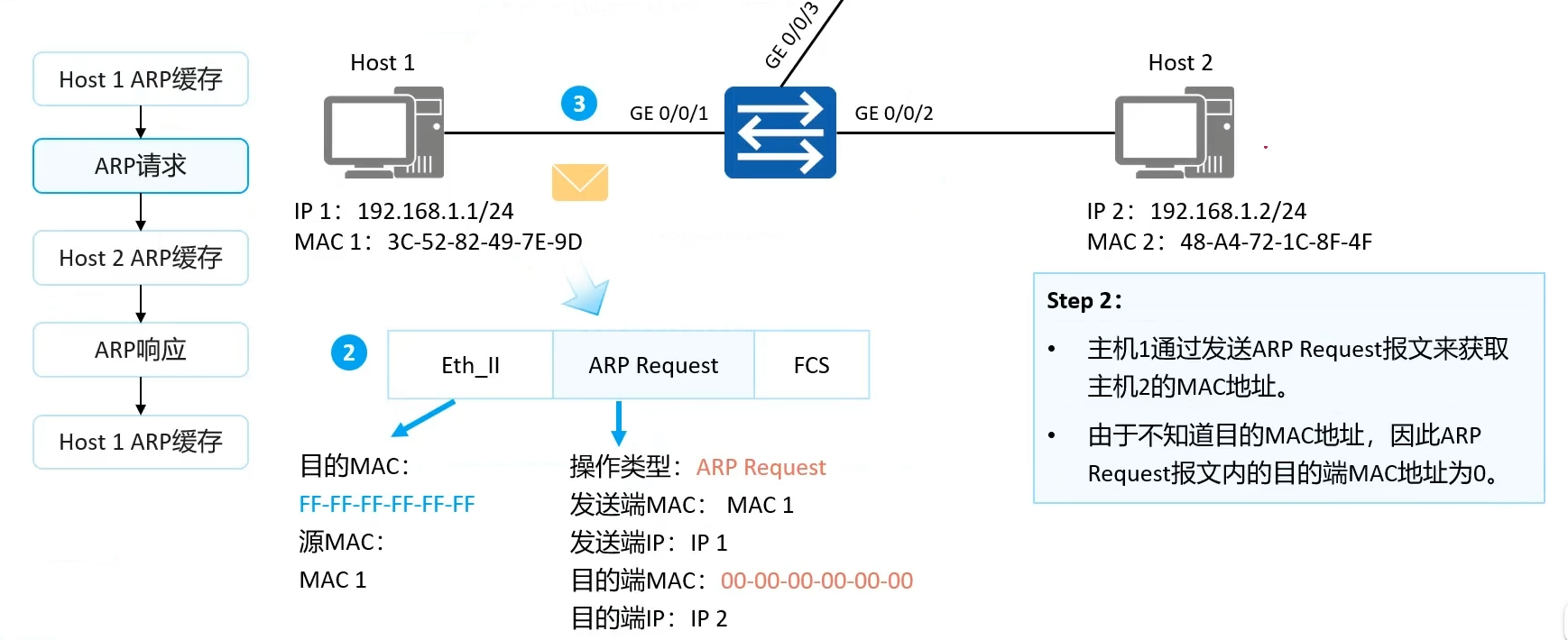
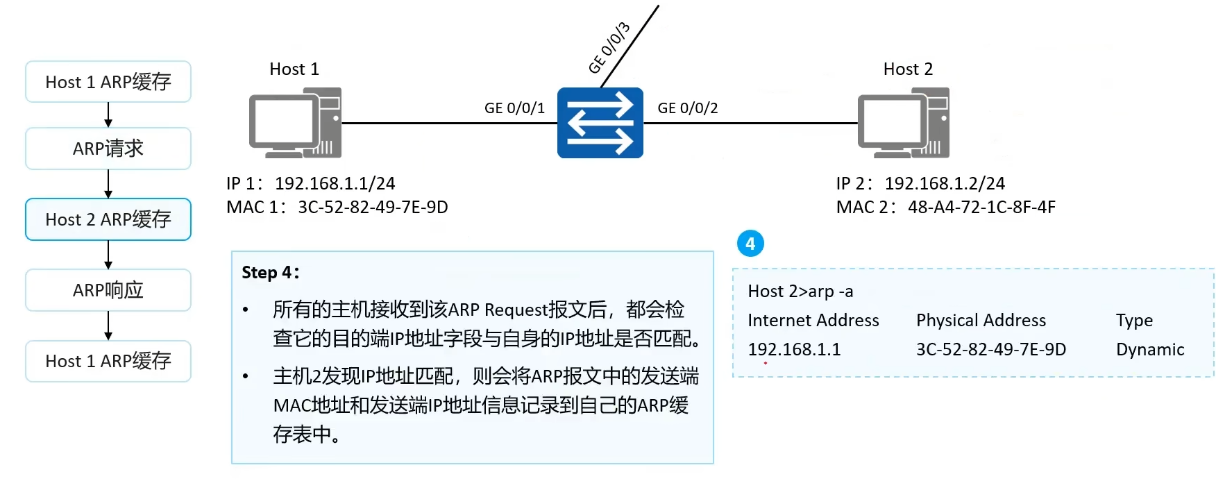
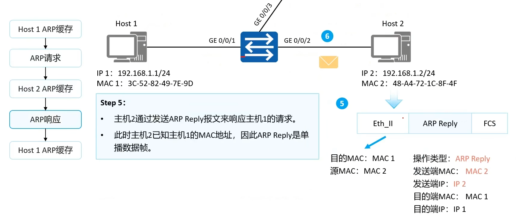
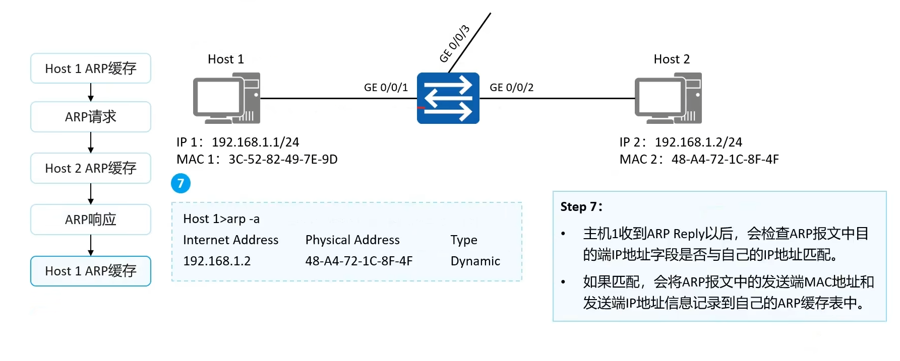
ARP Principle
- HOST1 ARP cache
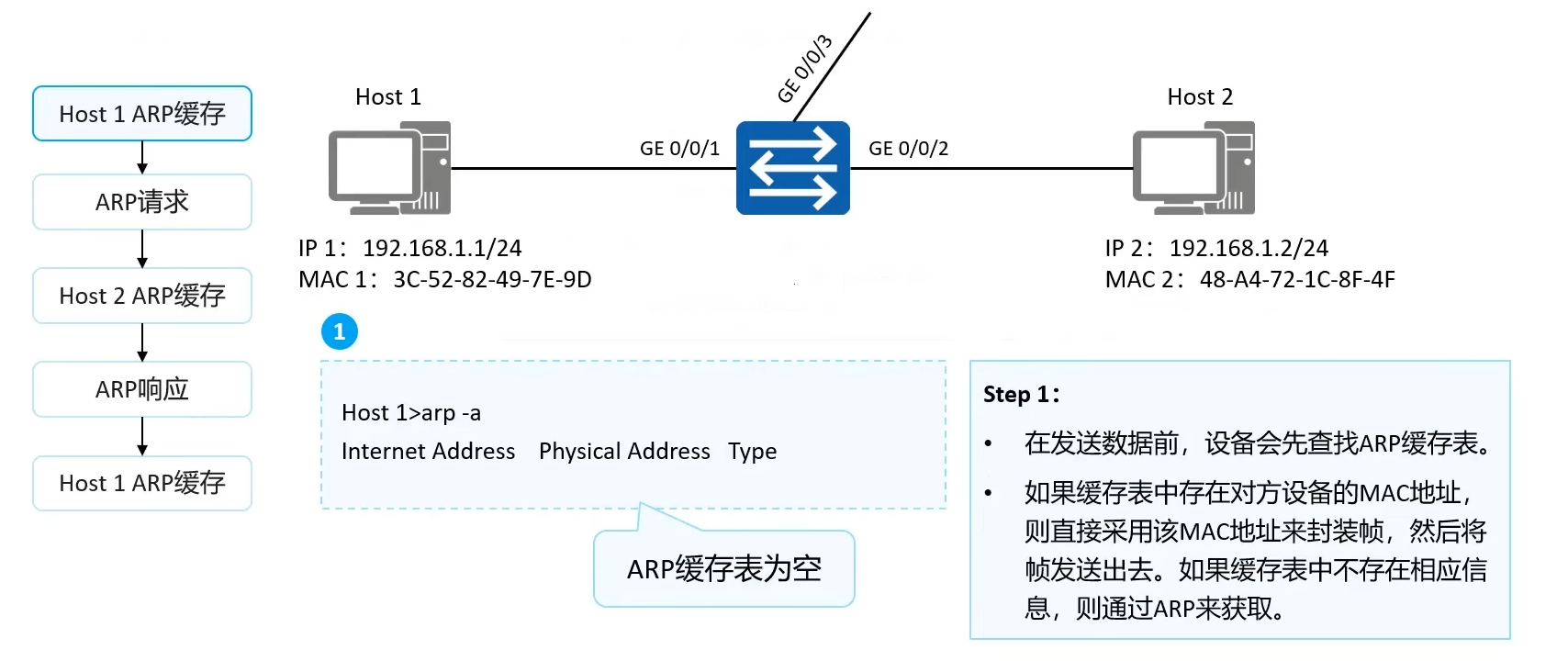
- ARP request
- HOST2 ARP cache — upon receiving, sends a unicast packet and saves it to the cache table
- ARP response — upon receiving, sends a unicast packet and saves it to the cache table
- HOST1 ARP response
IP Protocol
IPv4 Packet Format
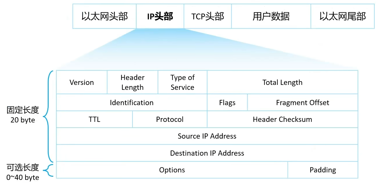
Packet Fragmentation
-
The process of dividing a packet into multiple fragments
-
IP packets forwarded over the network can vary in length, but when a packet's length exceeds the maximum length of the data link layer, it must be divided into several smaller fragments for transmission
- The data link layer has an
MTU(Maximum Transmission Unit); Ethernet defaults toMTU=1500 bytes
- The data link layer has an
Flag Bits
-
Identification
- All fragments split from the same original packet have identical identification values; the receiver uses it to determine which fragments belong to the same large packet
-
Flags (3 bits, only the last 2 bits are used)
-
MF bit (More Fragment)
-
1 = there are more fragments after this one
-
0 = this is the last fragment
-
The other bit: the
Don't Fragment bit. When set to 1, fragmentation is not allowed; an oversized packet is dropped directly and an ICMP error message is returned
-
-
Fragment Offset
-
8 bytes
-
Indicates: how many 8-byte units the data portion of the current fragment is offset from the start of the original packet
-
Used for ordering and reassembly
-
Except for the last fragment, all other fragment lengths must be
an integer multiple of 8 bytes -
The fixed 20 bytes of the IP header (with no options field) must be excluded when calculating, i.e.,
1480 bytes
-
-
Each fragment has its own IP header (the header is unchanged, only the data is split)
-
During routing and forwarding, fragments may travel over different paths and arrive out of order; the receiver relies on
identification + fragment offsetto sort and reassemble them
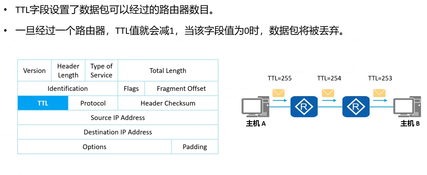
Time To Live (TTL)
-
An 8-bit field in the IPv4 header. Values: 0~255
-
Limits the maximum number of routing hops a packet can traverse; used to prevent loops
IP Classes
| Class | Leading Bits | First Octet Decimal Range | Default Subnet Mask | Network Bits | Host Bits | Primary Use |
|---|---|---|---|---|---|---|
| A | 0 | 1 ~ 126 | 255.0.0.0 | 8 | 24 | Large networks |
| B | 10 | 128 ~ 191 | 255.255.0.0 | 16 | 16 | Medium networks |
| C | 110 | 192 ~ 223 | 255.255.255.0 | 24 | 8 | Small LANs |
| D | 1110 | 224 ~ 239 | — | — | — | Multicast |
| E | 1111 | 240 ~ 255 | — | — | — | Research / Reserved |
| Private IP addresses that can be freely used on the intranet, not consuming public addresses: |
-
Class A private range:
10.0.0.0 ~ 10.255.255.255 -
Class B private range:
172.16.0.0 ~ 172.31.255.255 -
Class C private range:
192.168.0.0 ~ 192.168.255.255
Routing
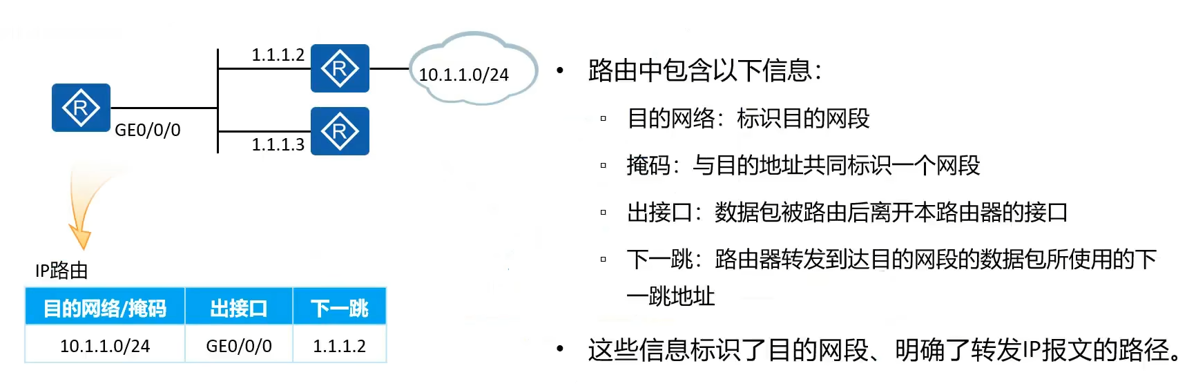
Route Acquisition Methods
-
Directly connected routes
- Automatically generated when devices are connected; priority 0, the highest
-
Static routes
- Manually configured; default priority 60
-
Dynamic routes
-
Devices automatically exchange route information with each other
-
Self-learning, self-updating
-
OSPF routes
-
Internal route priority 10
-
External route priority 150
-
-
Static route configuration rule:
ip route-static
{next-hop IP | outgoing interface | next-hop + outgoing interface}
Equal-Cost Routes
Definition: For the same destination network, multiple routes have exactly equal cost metrics, and the router forwards traffic across multiple links simultaneously
When the following three conditions are met, the routing table generates multiple route entries at the same time, enabling equal-cost load sharing. Prerequisites:
-
The destination IP network is the same
-
The cost calculated by the routing protocol is the same
-
The next hops and outgoing interfaces differ (two or more different physical paths exist)
Floating Static Routes
Definition: For the same destination network, two static routes are configured; the primary route has a higher priority, while the backup route with a lower priority does not enter the routing table. When the primary link fails, the backup automatically takes over
Key points:
-
Huawei / H3C: the smaller the priority value, the more preferred; Cisco is also the smaller the more preferred
-
Default static priority is 60
-
Floating backup route setting: 61~255 (the larger, the lower the priority)
OSPF
Definition
Definition: Open Shortest Path First, a classless inter-domain routing protocol, belonging to the IGP (Interior Gateway Protocol) and link-state routing protocols. Based on the SPF algorithm
-
Protocol number:
89 -
Multicast addresses:
224.0.0.5(all OSPF routers),224.0.0.6(DR/BDR) -
Features:
classless, supportsVLSM, supportsroute summarization,fast convergence,loop prevention; suitable for medium-to-large campus / carrier intranets -
LSDB(Link-State DataBase): the "whole-network topology map" shared by all routers within the same OSPF area, storing all LSA entries of the area.
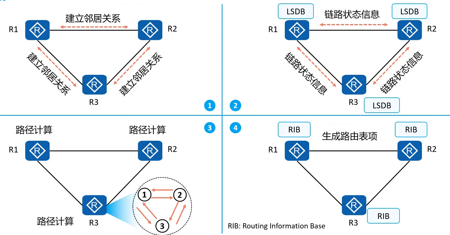
OSPF Principles
-
A link-state IGP protocol with IP protocol number 89; routers do not exchange routes directly with each other, but send each other LSA (link-state advertisement) messages describing links, costs, and neighbors
-
Routers within the same area fully synchronize an identical LSDB (link-state database)
-
Neighbors discover and maintain each other through Hello packets; after negotiation succeeds, LSAs are exchanged, and the LSDB reaches a Full adjacency
-
Each router runs the SPF algorithm rooted at itself, independently computing the shortest paths based on the LSDB to generate its routing table
-
Areas are divided into the backbone Area 0 and non-backbone areas; the purpose is to reduce the scope of LSA flooding; ABRs are responsible for inter-area route propagation
-
Broadcast networks elect DR/BDR to reduce the number of adjacencies
-
Cost is used as the metric, defaulting to
10^8/interface bandwidth -
Different types of LSA handle inter-area, intra-area, and external routes; LSAs are flooded within their specified scope
The Functions and Establishment Process of OSPF's 8 States
State order: Down → Attempt → Init → 2‑Way → ExStart → Exchange → Loading → Full
Among them, Attempt appears only in NBMA networks (Frame Relay)
The complete interaction of the 8 states is as follows:
-
Down
- If no Hello packet has been sent yet, it remains in the Down state
-
Attempt
- Neighbors are manually configured; Hello packets are sent by unicast, waiting for a response from the peer
-
Init
-
After receiving a Hello packet, OSFP starts running and enters the Init state
-
Mainly to discover the peer and learn its link information, cost, neighbor information, etc.
-
For example: R1 sends a Hello packet to R2; R2 receives the Hello packet, sees
the peer's Router-IDin it, and after learning the peer's relevant information,R2 replieswith a Hello packet, writingR1's RIDand related information into its neighbor list;R1 receivesthe packet, seesits own RID in the neighbor list, and enters 2-Way; at this point R1also needsto send a Hello packetcarrying R2's RID;R2 receivesthe packet, sees its own RID, and R2enters 2-Way -
This process requires both sides to receive each other's Hello packets; a bidirectional neighbor relationship is established
-
Router‑ID is just an identity; the neighbor list field is the credential for bidirectional confirmation.
-
-
2-Way
-
Received a Hello packet, and the neighbor list in the Hello packet contains itself: bidirectional connectivity is established, and the neighbor relationship is formed.
-
After 2-Way, broadcast networks perform DR/BDR election; p2p networks skip it
-
Routers that are neither DR (Designated Router) nor BDR (Backup Designated Router) are called DRother
-
DRothers stay only at 2‑Way and do not proceed further
-
Devices that need to establish adjacency enter ExStart, e.g., DRother ↔ DR; DRother ↔ BDR
-
-
ExStart
-
After entering ExStart, LSDB synchronization begins; DBD packets are exchanged to elect the master/slave, typically the device with the larger Router‑ID becomes the master; it controls the DBD packet sequence numbers. Only master/slave is negotiated; no LSA summaries are exchanged.
-
After the master/slave is confirmed, it enters ExChange
-
-
ExChange
- After entering ExChange,
DBDpacketscarrying LSA summariesare exchanged. Each side tells the other which LSAs are in itsLSDB; only LSA summaries are passed, not complete LSAs
- After entering ExChange,
-
Loading
-
Comparing DBD summaries, when a router finds it lacks certain LSAs, it starts sending LSR packets to request the complete LSAs
-
The peer replies to the LSR request with LSU packets (carrying the complete LSAs); after receiving them, it also replies with LSAck acknowledgments
-
Repeatedly request, update, and acknowledge
-
-
Full
-
When all LSAs are synchronized and the LSDB databases are consistent, the SPF algorithm starts running to compute routes, and the adjacency completes, entering the Full state
-
A complete OSPF routing table is generated. Note: each router has its own global routing table; neighbors do not pass route entries to each other, only LSA topology, and each computes its own routes. Among them, the LSA aging time is one hour
-
When there is no failure, Hello (10s) packets maintain the relationship; a Hello is sent every 10 seconds to ensure the neighbor is still alive
-
When four consecutive Hello packets go unanswered, there is a Dead Time of 40 seconds timer, i.e., the maximum allowed timeout for the neighbor: four Hello packet intervals. When the timer expires, the neighbor is judged to have failed; the neighbor and all LSAs learned from it are deleted, SPF computation restarts, and the state is reset to Down
-
When the network changes, an LSA with an updated version number is generated and flooded across the entire network using LSU packets; however, different LSA types have restricted propagation scopes, flooding only within the corresponding scope each LSA can reach — see the LSA classification for details
-
Routers receiving the LSU compare it against their LSDB, update their local LSDB, and reply with LSAck acknowledgment
-
Trigger SPF recalculation (not a full recomputation) to refresh the OSPF routing table
-
The neighbor state remains Full and does not fall back to ExStart; it only regresses when the neighbor fails and disconnects
-
-
OSPF Areas
The concept of area division: if the entire network is not divided and only Area 0 exists, all devices would share a single LSDB, making the network too large; it would also produce a huge number of LSAs, causing repeated full-network SPF runs and frequent network flapping
LSA Classification
| Number | Common Name | LSA Name | Generator | Flooding Scope | Core Function |
|---|---|---|---|---|---|
| Type‑1 | Type 1 LSA | Router LSA | Every router in the area | Local area | Describes all directly connected links and costs of the router; source of intra-area routes |
| Type‑2 | Type 2 LSA | Network LSA | DR of the broadcast segment | Local area | Describes broadcast / NBMA multi-access segments, listing all routers on the segment |
| Type‑3 | Type 3 LSA | Summary‑Network LSA | ABR | Other areas | Propagates routes between different areas, inter-area routes O IA; supports route summarization |
| Type‑4 | Type 4 LSA | Summary‑ASBR LSA | ABR | Other areas | Advertises the Router‑ID location of the ASBR router, serving Type 5 external routes |
| Type‑5 | Type 5 LSA | AS‑External LSA | ASBR | Entire OSPF AS | Introduces external routes (static, other protocols); E1/E2 two metrics |
| Type‑6 | Type 6 LSA | Group‑Membership LSA | MOSPF router | Local area | Used by MOSPF multicast OSPF; not used by ordinary unicast OSPF |
| Type‑7 | Type 7 LSA | NSSA‑External LSA | ASBR within the NSSA area | NSSA area only | NSSA area introduces external routes; NSSA‑ABR converts Type 7 to Type 5 LSAs; N1/N2 |
| Type‑8 | Type 8 LSA | External‑Attribute LSA | ASBR | Entire AS | Carries external route attributes such as BGP; barely used in live networks |
| Type‑9 | Opaque LSA #9 | Opaque‑LSA (link-local) | Router | Local link only | Extension features; cannot flood across routers |
| Type‑10 | Opaque LSA #10 | Opaque‑LSA (area scope) | Router | Local area | MPLS‑TE, Segment Routing; floods within the local area |
| Type‑11 | Opaque LSA #11 | Opaque‑LSA (entire AS) | Router | Entire AS domain | Extensions such as SR; floods across the whole OSPF domain |
Backbone Area
Area 0 definition:
-
Exists and is unique; the backbone area -
All normal areas
must be directly connected to Area 0; areas cannot be daisy-chained onto other areas (Area 1 connecting to Area 2 without connecting to Area 0 is an incorrect topology) -
Non-backbone areas that are
isolatedand cannot directly connect to Area 0 must configure a virtual linkVirtual-linkto reach the backbone
Area 0 function: after each area's routes are summarized, they are forwarded through the backbone, acting as the high-speed backbone of the entire OSPF network
Non-Backbone Areas
Areas 1 through N are non-backbone areas
Features: when the topology changes in this area, LSAs do not leave the area, and other LSDBs are not affected
IR (Internal Router) definition: all interfaces are entirely within the same Area (all in Area 0 or all in Area 1), without crossing areas
ABR (Area Border Router) definition: one side is Area 0 and the other is a normal area; generates Type 3 summary LSAs; responsible for inter-area routes
ASBR (Autonomous System Boundary Router) definition: when an ABR device introduces external routes such as static routes, RIP, BGP, it becomes an ASBR; generates Type 5 LSAs (NSSA generates Type 7, converted to Type 5 when leaving the area)
Special Areas
Normal standard area:
Types 1, 2, 3, 4, 5 LSAsall exist
Special areas are used toblock external Types 4 and 5 LSAs; the ABR automatically advertises adefault routeto replace the huge number of specific routes
Reference detail table:
+++ info\
| Special Area Type | LSAs Allowed to Keep | LSAs Forbidden | Core Optimization Effect |
|---|---|---|---|
| Normal standard area | All of Types 1/2/3/4/5 | None | Full routing capability, no optimization |
| Stub area | Types 1/2/3 (detailed) + default Type 3 route advertised by ABRA | Types 4 and 5 external LSAs | Blocks a large number of external routes from outside the domain, streamlining the LSDB |
| Totally Stub area | Types 1/2 + default Type 3 route advertised by ABR | Type 3 (detailed), Types 4, 5 | Extremely streamlined LSDB, keeping only intra-area topology + default exit route |
| NSSA area | Types 1/2/3 (detailed) + local Type 7 external LSAs + default Type 3 route advertised by ABR | Incoming external Types 4 and 5 LSAs | Blocks external routes from outside the domain while allowing the area to introduce local external routes |
| Totally NSSA area | Types 1/2 + local Type 7 external LSAs + default Type 3 route advertised by ABR | Type 3 (detailed), incoming Types 4, 5 | Extremely streamlined + local external network access capability; first choice for branch sites |
| ;;; |
| Area Type | LSAs Present | Characteristics |
|---|---|---|
| Standard normal area | 1, 2, 3, 4, 5 | Has Types 4 and 5, no Type 7 |
| Stub | 1, 2, 3 (no 4, 5) | No 4 or 5; ABR advertises a default Type 3 |
| Totally Stub | 1, 2 + default Type 3 | No detailed Type 3, no 4 or 5 |
| NSSA | 1, 2, 3, 7 (no incoming 4, 5) | Has Type 7; no external Type 5 enters the area |
| Totally NSSA | 1, 2, 7 + default Type 3 | No detailed Type 3, no incoming 4 or 5 |
| ;;; | ||
| +++ |
Stub Area
-
Removed:
Types 4 and 5 LSAs; keepTypes 1, 2, 3 -
The ABR
advertisesadefault Type 3 route -
No ASBR is allowed; no external routes can be introduced, so there is neither Type 5 nor Type 7
Totally Stub Area
-
Removed:
Type 3(except the default),Types 4 and 5 LSAs; onlyTypes 1 and 2+ adefault routeremain -
Small LSDB; first choice for branch sites
NSSA Area
-
An
ASBR may exist, and the area is allowed tointroduce external routes(generatingType 7 LSAs) -
Filters external Types 4 and 5 LSAs; the ABR advertises a default route -
The ABR
convertsType 7 LSAs into Type 5 LSAs and sends them to the backbone area and other areas; Type 7 can onlyflood within the NSSA areaandcannotleavethe NSSA
Totally NSSA Area
-
Removed:
Type 3(except the default),Types 4 and 5 LSAs; localexternal Type 7 LSAs are kept -
Optimal: the first choice when small branches need external network access and streamlined routing
Distance Vector vs. Link-State
Distance Vector
-
Sends the routing table to neighbors, and neighbors compute routes based on that table; it is "hearsay" — trusting what the neighbor says
-
Representative protocols: RIP, IGRP, EIGRP (Cisco)
-
RIP has a maximum of 15 hops; 16 hops is unreachable. Advantages: simple configuration, small memory footprint, suitable for small networks. Disadvantages: prone to loops — the repeated sending of the routing table wastes bandwidth; hop count is used as the metric, ignoring link bandwidth, so high- and low-speed links incur the same cost and route selection is unreasonable
Link-State
-
Only sends information about its own directly connected links; each router across the network draws the shortest paths independently, which is "actual measurement" — each draws its own map in real time
-
Representative protocols: OSPF, IS-IS
-
Advantages:
-
Almost no routing loops; LSA flooding (link-state advertisement) is sent only when links change, and incremental updates save bandwidth
-
Bandwidth, delay, etc. are used as metrics, giving precise route selection; suitable for large networks
-
-
Disadvantages:
-
High resource consumption; demanding device requirements
-
Complex configuration; requires dividing areas: Area, DR/BDR, etc.
-
How Switches Work
Layer 2
- MAC learning — when a switch receives a data frame, it reads the source MAC address in the frame header:
-
If the MAC address table does not have this MAC, write "receiving port + source MAC" into the MAC address table;
-
If it already exists, update the corresponding port and aging time;
Only the source MAC is used for learning; the destination MAC is used to decide forwarding.
- Frame forwarding/unicast — take the destination MAC address of the frame and look it up in the MAC address table:
-
✅ MAC found in the table: forward directly out the corresponding port, not to other ports (isolating traffic).
-
❌ MAC not found in the table: perform flooding (broadcast forwarding), forwarding the frame to all ports except the receiving port.
-
Broadcast/multicast frames
When the destination MAC is the broadcast addressFF‑FF‑FF‑FF‑FF‑FF, the switch directly floods to all ports, and all ports receive the broadcast. -
Aging and deletion
MAC address table entries have an aging time (default 300 seconds); if no packets from the device are received for a long time, the entry is automatically deleted to prevent table overflow.
Layer 3
Layer 2 only looks at MAC; Layer 3 switches add IP routing capability and can perform inter-VLAN forwarding based on IP.
::: success
Study tip: learn from the source MAC, look up the destination MAC; if found, unicast forward, if not found, flood; broadcast frames go to all ports, and entries aged out on timeout are deleted.
:::
VLAN
The core idea is that devices in the same broadcast domain can communicate; the main port types are access, trunk, and hybrid
Used to prevent broadcast domains from growing too large and to isolate broadcast domains
-
access: mainly connects to end devices; it strips the tag before sending frames to the end device
-
trunk: mainly connects to the same type of device; it carries VLAN tags when sending frames to other switches and allows multiple VLANs to pass. Only the PVID (native VLAN) strips the tag
-
hybrid: combines the features of access and trunk; you can manually specify which VLANs are tagged and which are stripped. Highly flexible
::: info
pvid vs. vid
port vlan id and vlan id, literally: vid is the VLAN's own number and belongs to the data frame; pvid is a port parameter — the VLAN number the port assigns to untagged frames — and belongs to the port configuration
-
Access PVID = the VID of the port's VLAN; when an untagged frame is received, it is tagged with this VID; when sent out, the tag of this VID is stripped.
-
Trunk PVID is the port's native VLAN; frames of the VID corresponding to the PVID have the tag stripped when sent; other VIDs keep their tags.
-
Hybrid The PVID is still used to tag untagged frames; whether to strip tags does not depend on the PVID — manual commands specify whether each VID is untagged
:::
If you enjoyed this, leave a comment~